Course: Graphical and Python programming using NAO
10: Finding Your Way

Solving Mazes
 
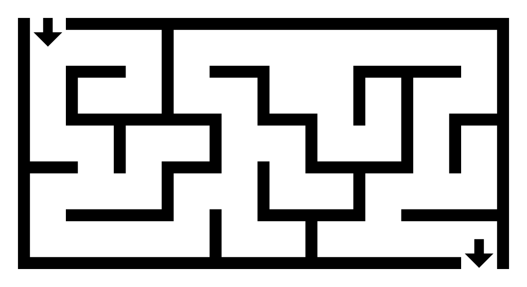
Many of us have had experience solving mazes on paper. The figure below, taken from the Wikimedia Commons, is one such maze. There is a defined start and goal, and we want to find a path from the start to the end. However, solving a maze on paper is somewhat different from solving a maze while you are in it. If you have walked in a hedge maze, you should know what it is like. For one thing, there is no map of the entire maze, so you don’t know beforehand if taking a left or right turn is the correct thing to do. Furthermore, it is difficult to keep track of where you have been in the maze, which can cause you to go around in circles.
 

 
There are many algorithms to help solve mazes. There are algorithms for cases where you know the map of the maze (such as when you do it on paper), and when you don’t (like when you are walking in a hedge maze). We will explore a number of these algorithms in this module, as we go through the exercises.
 
 
 
Dead-End Filling
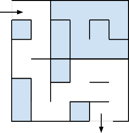
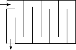
One algorithm to solve a maze when you have the map is called dead-end filling. Essentially, the idea is to find dead ends in the maze, and fill it up. This process repeats until no more dead ends exist. The remaining squares then form the solution from the start to the goal. In the figure to the left, the dead ends of the maze are shown with dots, and on the right, those dead ends have been filled, creating new dead ends which are shown with new dots. When the process of filling all the dead ends are completed, the resulting maze is shown at the bottom, which corresponds to the solution path.
 

 
 

Basic Task: Maze Solving with Visual Cues
 
In this exercise, the NAO will be placed in a maze, and the goal is for the NAO to walk from the start to the end. To do so, we can make use of the human brain to solve the maze. We will then use visual cues to help the NAO navigate the maze. Cues are objects or events that provide information and instruction for the NAO. Visual cues are cues that are detected by vision, such as a NAOMark.
 

1. With the map of the maze, find a path from the start position to the goal. The figure below shows a maze and the path. Do this on the maze map that you have been provided with. You can use the dead-end filling algorithm described above.  

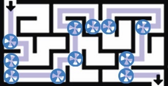
2. In addition to the map of the maze, you should have been given a number of NAOMarks. You can place these visual cues in the maze to instruct the NAO what to do. For example, In the figure below, NAOMarks are placed at every junction that the NAO should make a left turn. 

 
 
 
3. Similarly, you can use a different set of NAOMarks to instruct the NAO to make right turns, as shown below. 

 

4. With both sets of NAOMarks in place, we can now program the NAO to complete the maze. Essentially, the NAO should walk forward if it doesn’t see a NAOMark. When a NAOMark is detected, it should turn 90 degrees to the left or to the right, depending on the identification number of the NAOMark. 


5. However, to see the NAOMark and make a turn, the NAO should make use of its bottom camera, instead of the top camera.

You now need to create a program using Choregraphe to get NAO to solve the maze and walk to the end of it. 

Now, by placing NAOMarks in the right places, you can give visual cues to the NAO in order to complete the maze! 

Run the program and test.
 
 
 
 

Intermediate Task: Maze Solving with Multiple Cues
 
Besides NAOMarks, object recognition can also be used as visual cues. Together, they provide actions for the NAO. We have previously covered learning object features into the object recognition library on the NAO and using the Object Reco box to control the NAO.
 
Besides visual cues, you can also make use of the other sensors on the NAO, such as the touch sensors on its head, and the foot bumpers on its feet. For example, touching the head could make the NAO walk forward a short distance, and hitting a foot bumper will make the NAO turn 90 degrees in that direction.
 
Audio cues can also be used. You can tell the NAO to “turn left”, “turn right” and “walk forward”.
 
In this exercise, like the exercise above , you will be given the map of the maze. You can solve the maze on paper before working on the NAO. The NAO does not need to solve the maze automatically. Instead, it uses cues to decide what actions to take.
 
You can provide any sort of cue to the NAO, such as visual, sensory or audio cues. The score of a team will be calculated as follows:

• +100 if the NAO reaches the goal position by navigating through the maze
• +30 for each new type of cue, e.g.,
• NAOMarks
• visual objects
• button presses
• speech recognition
• face recognition
• +1 for every second under 5 minutes

 
For example, a team that only uses NAOMarks to complete the task in 4 minutes will have a score of 100 + 30 + 60 = 190. Another team that uses all 5 types of cues, and completes the maze in 4 minutes and 35 seconds will achieve 100 + 5 * 30 + 25 = 280.
 
As such, there is an incentive to develop an algorithm that is fast to execute and is less susceptible to errors.
 
 

Solving a Maze without a Map
 
We will now explore an algorithm that can be used when the map of the maze is unknown. For example, a person physically walking in a hedge maze can use it. Similarly, the algorithm can be used by a robot in a maze. The algorithm has a straightforward concept - as you walk in the maze, keep one of your hands, say the right hand, in contact with a wall of the maze at all times. Thus, when there is a turn to the right, in order to maintain contact with the right turn, the algorithm will take the right turn. In this fashion, the algorithm is guaranteed to find the exit provided a condition is met. The condition is that all the walls of the maze are connected together or to the boundary of the maze. This is also known as a simply connected maze.
 
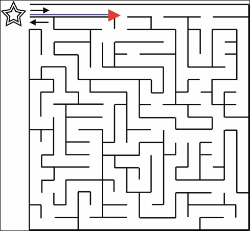
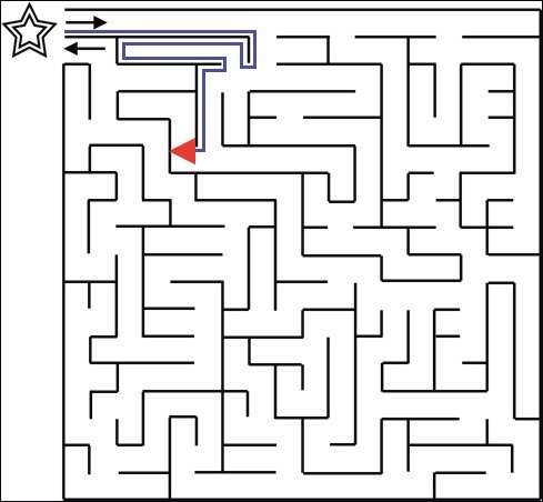
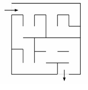
In the figures below, the algorithm will be performing the right-hand-rule, i.e., keeping the right side in contact with a wall. The parts of the walls that have been in contact are highlighted in blue.
 
In this first figure, the algorithm follows the right wall, up until the first junction.
 

 
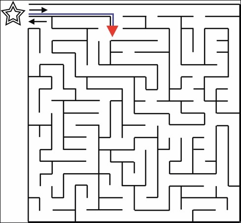
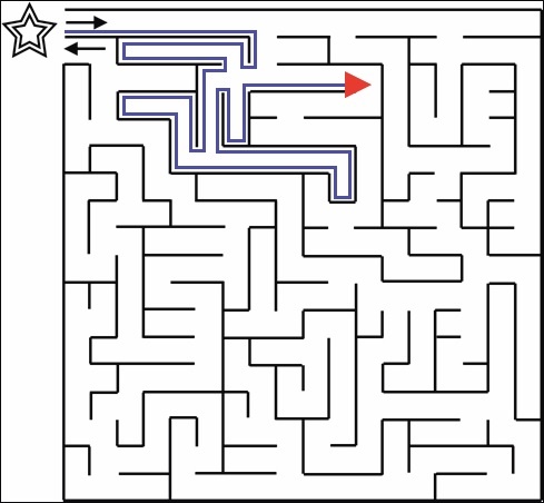
Since the right wall makes a turn, the algorithm will continue following the right wall and so it turns right. After making the first right turn, the algorithm follows the wall again to reach a new junction. Here, the algorithm continues to follow the wall, and go around the junction.
 

 
 
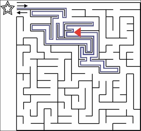
The algorithm continues on and follows the right wall whenever it makes a turn. The following four figures show the state of the algorithm as it keeps going.
  
      

     
 
Eventually, the algorithm reaches the goal position and completes.
 

 
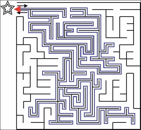
As you can see from the figure above, the algorithm takes a very long path from the start to the goal. However, while there are other algorithms that work when the map of the maze is not available, the wall-following algorithm is one of the easiest to implement.
 
 

Advanced Task: The Right Way to Maze Solving
 
In the previous two tasks, you were given the map of the maze, and gave cues for the NAO to walk from the start position to the goal. In this exercise, you will not be given the map of the maze. Instead, the NAO has to explore the maze and find its way to the goal automatically.
 
We will be using the Wall Following algorithm in order to do this, and we will use the right-hand-rule. The algorithm can be performed as follows:

1. If there is no wall to the right, turn 90 degrees to the right and then walk forward.
2. If there is a wall to the right, but no wall in front, then walk forward.
3. If there is a wall to the right, and a wall in front, then turn 90 degrees to the left.

 
In order for the algorithm to function, the NAO needs to know the state of the environment around it, i.e., whether there are walls to its right and/or in front of it. The state can be detected through a variety of methods, such as visual cues, audio, and sensors. We will leave it to you to decide what sort of cues you want to use for this module.
 
In the instructions below, we will be using the head touch sensor to inform the NAO about the state of the environment. Tapping the front head button indicates that there is a wall in front of it, and tapping the rear head button indicates that there is a wall to the right. Tapping the middle button means that the input is done, and the NAO should execute the next action.
 
Thus, if we only tapped the middle button, then there are no walls on the right and front of the NAO. If we tapped the top then middle button, then there is a wall to the front, but none on the right. If we tapped the rear then middle button, there is a wall to the right, but not the front. And lastly, if we tapped the front, rear, and then the middle button, there are walls to the front and the right.
 
Once the state of the environment is known, the NAO can then execute the correct action.
 
1. First, we will use the Tactile Head box from the Sensors category, to detect touches on the head.

2. Now, create a custom Python box, and add 3 inputs of type “bang”. 

 
 
3. Connect each of the outputs of the Tactile Head box to the inputs of the custom Python box. Then, double-click the Python box to edit the code. 

 

4. First, in theonLoad function, initialize a few variables. We create a proxy to ALMotion, and 2 boolean variables, front and rear, to store whether the front and rear head touch sensors were triggered. Also, forwardDist stores the distance in meters that the NAO should walk to move from one node in the maze to another. 

 
 
 
5. Next, edit the 3 functions that are triggered by the Python box’s inputs, onInput_Front, onInput_Middle and onInput_Rear. The code for onInput_Front and onInput_Rear set the relevant boolean variables to True, to indicate that a wall is present in front and to the right of the NAO respectively. When the middle button is triggered, the algorithm computes the next action for the NAO and executes it. Then, the variables storing the states of the walls are reset to False. 

 

6. Finally, the function computeAction needs to be filled in. In this function, the different cases of the walls are checked, and the relevant action is taken.

Implement the algorithm presented above.

7. Run the behavior without putting the NAO in the maze. Try pressing the head buttons and check that the NAO performs the correct action. 
​​
8. Now, place the NAO in the maze. Touch the head sensors to indicate whether there is a wall to the front and/or right of the NAO, and ensure that the NAO successfully executes the wall-following algorithm and reaches the goal position.

Finding the Shortest Path in a Maze
 
Another algorithm to solve a known maze is called breadth-first search. The search algorithm visits cells in a queue data structure (discussed in an earlier module), and adds neighboring cells into the queue as it goes along. By exploring the maze in this fashion, the algorithm is guaranteed to find the shortest path from the start to the goal.
 
The algorithm can be described with the following steps:

1. Add the starting position into the queue, and give it a value 1.
2. Remove the front node from the queue, and save its value as i.
3. If the node is the goal position, go to step 7.
4. Otherwise, examine all the neighbors of that position. If the neighbor hasn’t been visited before, add it into the queue with value i + 1.
5. If the queue is empty, there isn’t a path from the start to the goal.
6. Otherwise, go to step 2.
7. The goal position has been found, and has value i.
8. Look at the neighbors of the node and pick one that has value i - 1.
9. Repeat step 8, reducing i  by 1 in each step, until the starting position is reached.
10. The order of nodes corresponds to the reverse of the path from the start to the goal.

 
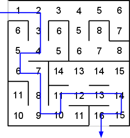
The figures below illustrate the steps in the algorithm, and the numbers over each node correspond to the value given to that node in the queue. We will describe how the algorithm proceeds using the figures. Numbers in red indicate nodes that are in the queue, and numbers in blue indicate nodes that were visited and are no longer in the queue.
 
Initially, the only node in the queue is the start position, and it has value 1. (Step 1)

 
The front node of the queue is removed (node 1), and its neighbors are examined. It has only 1 neighbor, and it is given a value 2, and placed in the queue. (Steps 2 to 6)
Note: Node 1 is no longer in the queue, and it is shown in blue in the figure below.
 

 
 
The process is repeated and more nodes are added into the queue. In the figure below, a node with value 8 has just been added to the queue. (Steps 2 to 6)
Note: Nodes with values 1-7 are no longer in the queue, but they are shown in the figure below.
 

 
Node 8 has two neighbors that have not been visited, so both of them get value 9 and are placed in the queue. (Steps 2 to 6)
 

 
 
 
The nodes with value 9 are removed from the queue one after the other, and their neighbors are given value 10 and placed in the queue. (Steps 2 to 6)
 

 
 
This process continues on as nodes are removed from the queue, and their neighbors are given higher values. The figure below shows the values of visited nodes up to 14, and the nodes in the queue with value 15. (Steps 2 to 6)
 

 
 
Eventually, the goal position receives a value of 100, and the algorithm jumps from step 3 to step 7. The figure below shows the values of the nodes on the path to the goal and their immediate neighbors. Not all the values of all explored nodes are shown. (Steps 2 to 7)
 

 
 
Now that the goal position has been reached, the path from the start position to the goal has to be found. To do so, we start from the goal position and store its value as i. In this case i = 100. From that state, we look at its immediate neighbors to find one with value i - 1, i.e., 99. There is only one neighbor with that value, so that node gets added to the final path. (Step 8)
 
In the figure below, the currently active node is highlighted in light blue, and its neighbors are shown in purple.

 
 
 
The algorithm now moves to the node with value 99. i is now set to 99 and the neighbors of the node is checked for i - 1. Again, there is only a single neighbor, so the algorithm selects that node. (Step 8)
 

 
 
The algorithm is now at the node with value 98, and so i = 98. The node has two neighbors that have not been considered, one with value 97 and one with value 99. Thus, the algorithm picks the node with value 97, i.e., i - 1. If there were more nodes with value 97, then it would not matter which node of value 97 the algorithm picked. (Step 8)
 

 
The algorithm continues in this fashion until the starting node is reached (value 1). The nodes that were selected by the algorithm along the way then form the path from the starting position to the goal. (Steps 9 to 10)
 
 
 

1. Complete the advanced task, without using Python.
   Hint: you can use a finite state machine to keep track of which buttons have been pressed.
2. Change the algorithm of the advanced task to do left-hand-following instead of right-hand-following.
3. Implement the breadth-first search algorithm in Python.
   

Questions
 
Basic: